Variance-component estimation with 1,000 individuals#
This tutorial repeats a seeded phenotype simulation ten times with 1,000 individuals. Each replicate samples raw dosage effects from the simplified evolutionary prior, adds residual noise, and estimates the variance components with profiled AI-REML. The final figure is a box plot of the ten estimates; the horizontal line in each panel is the generating value.
The example uses a broad, fixed allele-frequency spectrum so that the
frequency-dependent tau parameter is visible in a modest simulation. The
same fitting call can consume a genotype representation graph (GRG)
[DeHaas et al., 2025] through the matrix-free BOLT-style API;
the dense construction here keeps the ten-replicate tutorial quick and makes
the simulation boundary easy to inspect.
Simulation and fitting code#
Show the simulation and fitting code
 1"""Ten-replicate, 1,000-individual variance-component tutorial."""
 2
 3from __future__ import annotations
 4
 5import matplotlib.pyplot as plt
 6import numpy as np
 7
 8from evo_lmm import EvolutionaryLmmOps, SimplifiedPrior, fit_reml
 9
10
11N_INDIVIDUALS = 1_000
12N_VARIANTS = 500
13N_REPLICATES = 10
14TRUE_PRIOR = SimplifiedPrior(sigma_b2=0.004, tau=2.0)
15TRUE_SIGMA_E2 = 0.35
16
17
18def fit_one_replicate(replicate: int) -> tuple[float, float, float, bool]:
19    """Simulate and fit one replicate, returning ``(sigma_b2, tau, sigma_e2, converged)``."""
20
21    rng = np.random.default_rng(1_000 + int(replicate))
22    population_frequencies = np.linspace(0.03, 0.5, N_VARIANTS)
23    dosage = rng.binomial(
24        2,
25        population_frequencies,
26        size=(N_INDIVIDUALS, N_VARIANTS),
27    ).astype(np.float64)
28    frequencies = dosage.mean(axis=0) / 2.0
29    ops = EvolutionaryLmmOps.from_dense(dosage, frequencies, model="simplified")
30
31    effects = rng.normal(
32        0.0,
33        np.sqrt(TRUE_PRIOR.effect_variances(frequencies)),
34    )
35    phenotype = ops.apply_model_x(effects) + rng.normal(
36        0.0,
37        np.sqrt(TRUE_SIGMA_E2),
38        size=N_INDIVIDUALS,
39    )
40    fit = fit_reml(
41        ops,
42        phenotype,
43        initial=TRUE_PRIOR,
44        exact=False,
45        trace_probes=64,
46        seed=2_000 + int(replicate),
47        max_iter=25,
48        cg_tol=1e-8,
49    )
50    return (
51        float(fit.prior.sigma_b2),
52        float(fit.prior.tau),
53        float(fit.sigma_e2),
54        bool(fit.diagnostics.converged),
55    )
56
57
58def run_replicates() -> np.ndarray:
59    """Return one row per replicate with estimates and a convergence flag."""
60
61    return np.asarray(
62        [fit_one_replicate(replicate) for replicate in range(N_REPLICATES)],
63        dtype=np.float64,
64    )
65
66
67def make_box_plot(results: np.ndarray) -> plt.Figure:
68    """Draw log-scale estimate boxes with the generating values overlaid."""
69
70    estimates = results[:, :3]
71    true_values = np.array(
72        [TRUE_PRIOR.sigma_b2, TRUE_PRIOR.tau, TRUE_SIGMA_E2],
73        dtype=np.float64,
74    )
75    labels = [r"$\sigma_b^2$", r"$\tau$", r"$\sigma_e^2$"]
76
77    figure, axes = plt.subplots(1, 3, figsize=(10, 3.8), constrained_layout=True)
78    for axis, label, values, true_value in zip(axes, labels, estimates.T, true_values):
79        positive_values = np.maximum(values, np.finfo(np.float64).tiny)
80        axis.boxplot(positive_values, tick_labels=["10 replicates"], showmeans=True)
81        axis.axhline(true_value, color="tab:red", linestyle="--", label="true value")
82        axis.set_yscale("log")
83        axis.set_title(label)
84        axis.grid(axis="y", alpha=0.3)
85    axes[0].legend(loc="best")
86    figure.suptitle("Variance-component estimates, N = 1,000")
87    return figure
88
89
90if __name__ == "__main__":
91    results = run_replicates()
92    figure = make_box_plot(results)
93    print("converged replicates:", int(np.count_nonzero(results[:, 3])))
94    print(results[:, :3])
95    if "agg" not in plt.get_backend().lower():
96        plt.show()
The script uses seeded Hutchinson trace estimates. The estimate of
sigma_e2 is usually tighter than the shape estimate tau because a
single phenotype vector contains less information about the frequency shape.
For that reason the panels use logarithmic y-axes and show all ten replicates,
including fits that land near the tau=0 boundary.
Replicate estimates#
The figure summarizes the ten replicate fits.
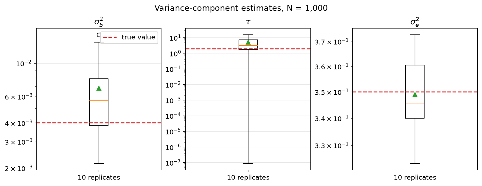
The box plot is a compact Monte Carlo diagnostic, not a replacement for
FitDiagnostics. In a real analysis, inspect convergence, trace standard
errors, AI conditioning, and boundary warnings alongside the point estimates.