Explicit forward simulation with SLiM

This tutorial uses SLiM to generate ten independent populations under the simplified evolutionary model, then fits evo-lmm to the sampled genotypes and phenotypes. Its purpose is to check the model in the setting from which its frequency-dependent prior is derived: mutation, drift, recombination, and stabilizing selection jointly determine which variants are segregating and their effects [Lee and Terhorst, 2026].

It is tempting to draw variant effects from the final conditional prior, simulate y = G beta + e, and fit the same model back to those data. That is a useful numerical check of the fitting code, but it is not a check of the evolutionary argument. In the model specification, the key step is the effect-dependent site-frequency spectrum p(G_j | alpha_j): stabilizing selection changes the chance that a mutation with a given latent effect is observed at a particular frequency. Conditioning that population process on the sampled genotype is what yields E[beta_j^2 | G_j]. A direct regression simulation assumes this relationship rather than generating it, and omits the finite-population and linkage effects that accompany it. Forward simulation therefore provides the appropriate end-to-end experiment.

The SLiM model follows the forward-simulation design described in [Lee and Terhorst, 2026]. Mutations have normally distributed latent effects, fitness is exp(-phenotype^2 / (2 * V_S)), and W_S = V_S / (2N) is the dimensionless selection-width parameter. This tutorial uses the simplified rho^2 = 1 case, for which the focal and selected effects agree: beta_j = alpha_j.

Prerequisites

SLiM is an external executable rather than a Python dependency of this project. Check that it is available before running the example:

slim -v

The project environment supplies tskit, pygrgl, and evo_lmm. The complete SLiM source is included as slim_simplified_prior.slim.

The forward model

The simulation fixes a diploid population of 2,000 individuals, runs for 10N = 20,000 generations across L = 10^6 bases, and records a tree sequence. It uses V_S = 2N = 4,000, hence W_S = 1. The complete SLiM source is included in the following expandable block.

Show the SLiM model

// Explicit forward simulation for the simplified evolutionary prior.
//
// This follows the m2/stabilizing-selection construction in:
// https://github.com/hanbin973/param_arch_stab_paper/blob/main/codes/scripts/burnin.slim
// and main.slim. Here m2 selection coefficients are the latent alpha effects.
// The simplified rho^2 = 1 specialization sets beta = alpha in Python.

initialize() {
    if (!exists("N")) defineConstant("N", 2000);
    if (!exists("L")) defineConstant("L", 1000000);
    if (!exists("MUT_RATE")) defineConstant("MUT_RATE", 1e-7);
    if (!exists("REC_RATE")) defineConstant("REC_RATE", 1e-8);
    if (!exists("SIGMA_A")) defineConstant("SIGMA_A", 1.0);
    // V_S is the fitness-landscape width. W_S = V_S / (2N) is the
    // dimensionless width used after diffusion-time rescaling.
    if (!exists("V_S")) defineConstant("V_S", 2.0 * N);
    if (!exists("W_S")) defineConstant("W_S", V_S / (2.0 * N));
    if (!exists("BURN_IN")) defineConstant("BURN_IN", 10 * N);
    if (!exists("OUTPUT_FILE")) defineConstant("OUTPUT_FILE", "slim_forward.trees");

    initializeTreeSeq();
    initializeMutationType("m2", 0.5, "n", 0.0, SIGMA_A);
    initializeGenomicElementType("g1", m2, 1.0);
    initializeGenomicElement(g1, 0, L - 1);
    initializeMutationRate(MUT_RATE);
    initializeRecombinationRate(REC_RATE);
}

1 early() {
    sim.addSubpop("p1", N);
    // The population mean is centered at the start, as in burnin.slim.
    defineConstant("INITIAL_MEAN", 0.0);
}

mutationEffect(m2) {
    // m2 coefficients are trait effects, not direct mutation fitness effects.
    return 1.0;
}

fitnessEffect() {
    phenotype = individual.sumOfMutationsOfType(m2) - INITIAL_MEAN;
    return exp(-1.0 * phenotype^2 / (2.0 * V_S));
}

BURN_IN late() {
    muts = sim.mutationsOfType(m2);
    sim.treeSeqOutput(OUTPUT_FILE);
    catn("Forward simulation complete: " + size(muts) + " m2 mutations");
    sim.simulationFinished();
}

SLiM records the mutation effects in tree-sequence metadata. The production scripts separate burn-in and replicate runs; this compact version combines the essential steps for a reproducible example.

SLiM to GRG to evo-lmm

For each replicate, the driver simplifies the extant samples with tskit, converts the tree sequence with pygrgl.grg_from_trees, computes sample allele frequencies, and uses the raw GRG dosage operator to form genetic values from the metadata-derived effects. The GRG is a compact, lossless representation that supports these graph-native operations [DeHaas et al., 2025]. The driver then adds residual noise and fits the simplified model. Simplification is needed because SLiM’s recording also marks historical nodes as samples.

Show the Python driver

"""SLiM -> tree sequence -> GRG -> evo-lmm simplified-prior check."""

from __future__ import annotations

from concurrent.futures import ThreadPoolExecutor
import json
from pathlib import Path
import subprocess
import tempfile

import matplotlib.pyplot as plt
import numpy as np
import pygrgl
import tskit

from evo_lmm import (
    EvolutionaryLmmOps,
    SimplifiedPrior,
    fit_evolutionary_bolt_lmm,
    sample_allele_frequencies,
)


N_INDIVIDUALS = 2_000
N_GENERATIONS = 10 * N_INDIVIDUALS
N_REPLICATES = 10
SEQUENCE_LENGTH = 1_000_000
SIGMA_A2 = 1.0
V_S = 2.0 * N_INDIVIDUALS
W_S = V_S / (2.0 * N_INDIVIDUALS)
TRUE_TAU = SIGMA_A2 / W_S
RESIDUAL_VARIANCE = 0.4
SEED = 812


def _simulation_manifest(seed: int) -> dict[str, int | float]:
    """Return the configuration that defines a persisted forward replicate."""

    return {
        "seed": int(seed),
        "individuals": N_INDIVIDUALS,
        "generations": N_GENERATIONS,
        "sequence_length": SEQUENCE_LENGTH,
        "sigma_a2": SIGMA_A2,
        "residual_variance": RESIDUAL_VARIANCE,
    }


def run_slim(output_directory: Path, seed: int = SEED) -> Path:
    """Run the checked-in SLiM script and return its tree-sequence file."""

    output_directory.mkdir(parents=True, exist_ok=True)
    tree_path = output_directory / "slim_forward.trees"
    if "__file__" in globals():
        script = Path(__file__).with_name("slim_simplified_prior.slim")
    else:
        # Keep this fallback for interactive execution from a source checkout.
        # Hosted documentation uses the pre-generated PNG assets instead.
        script = Path("docs/tutorials/slim_simplified_prior.slim")
        if not script.exists():
            script = Path("slim_simplified_prior.slim")
    script = script.resolve()
    subprocess.run(
        [
            "slim",
            "-s",
            str(seed),
            "-d",
            f"N={N_INDIVIDUALS}",
            "-d",
            f"L={SEQUENCE_LENGTH}",
            "-d",
            f'OUTPUT_FILE="{tree_path}"',
            "-d",
            f"BURN_IN={N_GENERATIONS}",
            str(script),
        ],
        check=True,
        cwd=output_directory,
    )
    return tree_path


def mutation_effects(tree_sequence: tskit.TreeSequence) -> np.ndarray:
    """Extract current SLiM m2 effects in tskit's mutation-row order.

    SLiM can stack recurrent mutations at one site. In that case, a tskit
    mutation row stores the current mutation first and its inherited mutation
    history after it; GRGL exposes one mutation column for the current row.
    """

    effects = []
    for mutation in tree_sequence.mutations():
        mutation_list = mutation.metadata.get("mutation_list", [])
        if not mutation_list:
            raise ValueError(
                "expected SLiM mutation metadata for every mutation row, "
                f"got none for mutation {mutation.id}"
            )
        effects.append(float(mutation_list[0]["selection_coeff"]))
    return np.asarray(effects, dtype=np.float64)


def _load_or_simulate_data(seed: int, output_directory: Path) -> dict:
    """Load one persisted simulation or create it in ``output_directory``."""

    output_directory = Path(output_directory).resolve()
    output_directory.mkdir(parents=True, exist_ok=True)
    simplified_path = output_directory / "slim_forward.simplified.trees"
    required = (
        simplified_path,
        output_directory / "alpha.npy",
        output_directory / "frequencies.npy",
        output_directory / "phenotype.npy",
        output_directory / "seed.txt",
        output_directory / "simulation.json",
    )
    try:
        recorded_seed = int((output_directory / "seed.txt").read_text(encoding="utf-8"))
    except (FileNotFoundError, ValueError):
        recorded_seed = None
    try:
        recorded_manifest = json.loads(
            (output_directory / "simulation.json").read_text(encoding="utf-8")
        )
    except (FileNotFoundError, ValueError, json.JSONDecodeError):
        recorded_manifest = None
    if (
        recorded_seed != int(seed)
        or recorded_manifest != _simulation_manifest(seed)
        or not all(path.exists() for path in required)
    ):
        tree_path = run_slim(output_directory, seed)
        recorded = tskit.load(str(tree_path))
        alpha = mutation_effects(recorded)
        # SLiM marks historical nodes as samples in its full recording. GRGL
        # expects the current haploid genomes to be the leaf samples, so use
        # ordinary tskit simplification before conversion. This is not PySLiM
        # annotation and preserves mutation order with filter_sites=False.
        tree_sequence = recorded.simplify(filter_sites=False)
        tree_sequence.dump(str(simplified_path))
        grg = pygrgl.grg_from_trees(str(simplified_path))
        frequencies = sample_allele_frequencies(grg)
        if alpha.size != grg.num_mutations:
            raise ValueError(
                "SLiM effect order does not match GRG mutation order: "
                f"{alpha.size} effects for {grg.num_mutations} mutations"
            )
        prior = SimplifiedPrior(sigma_b2=SIGMA_A2, tau=TRUE_TAU)
        ops = EvolutionaryLmmOps(grg, frequencies=frequencies, model="simplified")
        # rho^2 = 1: the focal effect beta is the selected-trait effect alpha.
        genetic_value = ops.apply_model_x(alpha)
        rng = np.random.default_rng(seed + 1)
        phenotype = genetic_value + rng.normal(
            0.0,
            np.sqrt(RESIDUAL_VARIANCE),
            size=ops.n,
        )
        np.save(output_directory / "alpha.npy", alpha)
        np.save(output_directory / "frequencies.npy", frequencies)
        np.save(output_directory / "phenotype.npy", phenotype)
        (output_directory / "seed.txt").write_text(f"{seed}\n", encoding="utf-8")
        (output_directory / "simulation.json").write_text(
            json.dumps(_simulation_manifest(seed), sort_keys=True) + "\n",
            encoding="utf-8",
        )
    else:
        tree_sequence = tskit.load(str(simplified_path))
        grg = pygrgl.grg_from_trees(str(simplified_path))
        alpha = np.load(output_directory / "alpha.npy")
        frequencies = np.load(output_directory / "frequencies.npy")
        phenotype = np.load(output_directory / "phenotype.npy")
        if alpha.size != grg.num_mutations:
            raise ValueError(
                "persisted SLiM effect order does not match GRG mutation order: "
                f"{alpha.size} effects for {grg.num_mutations} mutations"
            )
    if frequencies.shape != (grg.num_mutations,):
        raise ValueError("persisted frequency vector does not match GRG mutations")
    return {
        "seed": int(seed),
        "tree_sequence": tree_sequence,
        "grg": grg,
        "frequencies": frequencies,
        "alpha": alpha,
        "phenotype": phenotype,
    }


def _fit_forward_data(data: dict) -> dict:
    """Fit the tutorial model to one already prepared simulation."""

    seed = int(data["seed"])
    prior = SimplifiedPrior(sigma_b2=SIGMA_A2, tau=TRUE_TAU)
    fit = fit_evolutionary_bolt_lmm(
        [("slim", data["grg"])],
        data["phenotype"],
        frequencies={"slim": data["frequencies"]},
        model="simplified",
        initial=prior,
        trace_probes=64,
        max_iter=30,
        cg_tol=1e-8,
        seed=seed + 2,
    )
    return {**data, "fit": fit}


def simulate_and_fit(seed: int = SEED, *, output_directory: Path | None = None):
    """Run or load one SLiM data set, convert it to a GRG, and fit the prior."""

    if output_directory is not None:
        return _fit_forward_data(_load_or_simulate_data(seed, output_directory))
    with tempfile.TemporaryDirectory(prefix="evo_lmm_slim_") as directory:
        return _fit_forward_data(_load_or_simulate_data(seed, Path(directory)))


def prepare_replicates(
    workers: int = 1,
    *,
    artifact_directory: Path,
) -> list[dict]:
    """Run or load the ten forward simulations without fitting them."""

    seeds = [SEED + replicate for replicate in range(N_REPLICATES)]
    artifact_root = Path(artifact_directory).resolve()
    artifact_root.mkdir(parents=True, exist_ok=True)

    def run(seed: int) -> dict:
        return _load_or_simulate_data(seed, artifact_root / f"seed_{seed}")

    if workers <= 1:
        return [run(seed) for seed in seeds]
    with ThreadPoolExecutor(max_workers=int(workers)) as executor:
        return list(executor.map(run, seeds))


def run_replicates(
    workers: int = 1,
    *,
    artifact_directory: Path | None = None,
) -> list[dict]:
    """Run independent SLiM replicates and fit the tutorial prior.

    ``workers=1`` preserves the simple sequential tutorial execution. Local
    documentation generation may use a small thread pool because each
    replicate owns its SLiM process and GRG objects.  When ``artifact_directory``
    is supplied, the simulation outputs are persisted for the benchmark.
    """

    if artifact_directory is None:
        with tempfile.TemporaryDirectory(prefix="evo_lmm_slim_replicates_") as directory:
            data = prepare_replicates(workers, artifact_directory=Path(directory))
            if workers <= 1:
                return [_fit_forward_data(item) for item in data]
            with ThreadPoolExecutor(max_workers=int(workers)) as executor:
                return list(executor.map(_fit_forward_data, data))
    data = prepare_replicates(workers, artifact_directory=artifact_directory)
    if workers <= 1:
        return [_fit_forward_data(item) for item in data]
    with ThreadPoolExecutor(max_workers=int(workers)) as executor:
        return list(executor.map(_fit_forward_data, data))


def load_simulation_replicates(artifact_directory: Path) -> list[dict]:
    """Load persisted forward simulations without rerunning the tutorial fits."""

    root = Path(artifact_directory).resolve()
    if not root.exists():
        raise FileNotFoundError(
            f"forward artifacts are missing in {root}; run the figure generator first"
        )
    missing = [
        root / f"seed_{SEED + replicate}"
        for replicate in range(N_REPLICATES)
        if not (root / f"seed_{SEED + replicate}" / "slim_forward.simplified.trees").exists()
    ]
    if missing:
        raise FileNotFoundError(
            "forward replicate artifacts are incomplete; missing "
            + ", ".join(str(path) for path in missing)
        )
    return prepare_replicates(workers=1, artifact_directory=root)


def local_linear_regression(
    x: np.ndarray,
    y: np.ndarray,
    query: np.ndarray,
    *,
    span: float = 0.4,
) -> np.ndarray:
    """Evaluate a log-frequency local-linear regression of ``y`` on ``x``.

    The bandwidth is adaptive: each query point uses the nearest ``span``
    fraction of observations with a tricube kernel. This empirical smoother
    is plotted separately from the evolutionary prior formula.
    """

    if not 0.0 < span <= 1.0:
        raise ValueError("span must be in (0, 1]")
    x = np.asarray(x, dtype=np.float64)
    y = np.asarray(y, dtype=np.float64)
    query = np.asarray(query, dtype=np.float64)
    valid = np.isfinite(x) & np.isfinite(y) & (x > 0.0)
    if not np.any(valid):
        raise ValueError("local regression requires positive finite x values")
    log_x = np.log(x[valid])
    observations = y[valid]
    neighbor_count = min(
        log_x.size,
        max(8, int(np.ceil(span * log_x.size))),
    )
    fitted = np.empty(query.size, dtype=np.float64)
    for index, point in enumerate(np.log(query)):
        distances = np.abs(log_x - point)
        bandwidth = np.partition(distances, neighbor_count - 1)[neighbor_count - 1]
        bandwidth = max(bandwidth, np.finfo(np.float64).eps)
        scaled = distances / bandwidth
        weights = np.where(scaled < 1.0, (1.0 - scaled**3) ** 3, 0.0)
        design = np.column_stack((np.ones_like(log_x), log_x - point))
        weighted_design = weights[:, None] * design
        normal = design.T @ weighted_design
        rhs = design.T @ (weights * observations)
        try:
            fitted[index] = np.linalg.solve(normal, rhs)[0]
        except np.linalg.LinAlgError:
            fitted[index] = np.average(observations, weights=weights)
    return fitted


def make_summary(results: list[dict]) -> plt.Figure:
    """Plot one effect spectrum and replicate-level fitted components."""

    representative = results[0]
    fit = representative["fit"]
    frequencies = representative["frequencies"]
    alpha = representative["alpha"]
    minor_frequencies = np.minimum(frequencies, 1.0 - frequencies)
    observed = np.square(alpha)
    segregating = minor_frequencies > 0.0
    plot_frequencies = minor_frequencies[segregating]
    plot_observed = observed[segregating]
    curve_frequencies = np.geomspace(plot_frequencies.min(), 0.5, 200)
    parametric = fit.prior.effect_variances(curve_frequencies)
    local = local_linear_regression(plot_frequencies, plot_observed, curve_frequencies)

    figure, axes = plt.subplots(1, 2, figsize=(10, 3.8), constrained_layout=True)
    axes[0].scatter(
        plot_frequencies,
        plot_observed,
        s=8,
        alpha=0.25,
        label=r"SLiM $\alpha_j^2$",
    )
    axes[0].plot(
        curve_frequencies,
        parametric,
        color="tab:red",
        linewidth=2,
        label=r"parametric fitted $E[\beta_j^2\mid x_j]$",
    )
    axes[0].plot(
        curve_frequencies,
        local,
        color="tab:purple",
        linestyle="--",
        linewidth=1.5,
        label="local linear regression",
    )
    axes[0].set_xlabel("sample minor allele frequency")
    axes[0].set_ylabel(r"effect square / variance")
    axes[0].set_title("Forward-simulated effect spectrum")
    axes[0].set_xscale("log")
    axes[0].legend(loc="best")
    axes[0].grid(alpha=0.3)

    labels = [r"$\sigma_b^2$", r"$\tau$", r"$\sigma_e^2$"]
    estimates = np.asarray(
        [
            [result["fit"].prior.sigma_b2, result["fit"].prior.tau, result["fit"].sigma_e2]
            for result in results
        ],
        dtype=np.float64,
    )
    true_values = [SIGMA_A2, TRUE_TAU, RESIDUAL_VARIANCE]
    axes[1].boxplot(
        estimates,
        tick_labels=labels,
        showmeans=True,
        meanprops={"marker": "^", "markerfacecolor": "tab:green", "markeredgecolor": "tab:green"},
    )
    positions = np.arange(1, len(labels) + 1, dtype=np.float64)
    for position, true_value in zip(positions, true_values):
        axes[1].hlines(
            true_value,
            position - 0.3,
            position + 0.3,
            colors="tab:red",
            linestyles=":",
            linewidth=2,
            label="generating value" if position == positions[0] else None,
        )
    axes[1].set_ylim(bottom=0.0)
    axes[1].set_title(f"N={N_INDIVIDUALS}, {N_REPLICATES} replicates")
    axes[1].grid(axis="y", alpha=0.3)
    axes[1].legend(loc="best")
    return figure


if __name__ == "__main__":
    results = run_replicates()
    for replicate, result in enumerate(results):
        print(
            f"replicate={replicate} mutations={result['grg'].num_mutations} "
            f"prior={result['fit'].prior} sigma_e2={result['fit'].sigma_e2} "
            f"diagnostics={result['fit'].diagnostics}"
        )
    make_summary(results)
    if "agg" not in plt.get_backend().lower():
        plt.show()

Run the simulation and fitting workflow with:

uv run python docs/tutorials/slim_forward_simplified.py

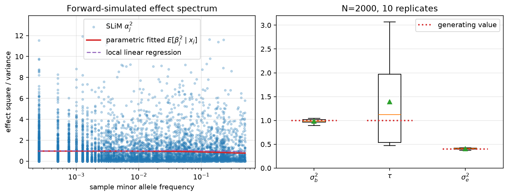
The fitted sigma_b2 and tau are finite-sample estimates, not exact recovery targets. Each replicate contains one finite genomic region and one phenotype vector, which leave limited information about the frequency-shape parameter even after the 10N-generation burn-in. Inspect FitDiagnostics before interpreting an individual fit.

Summary figure

The script produces a two-panel summary. The left panel compares realized alpha_j^2 values among segregating variants in the first replicate with two summaries on the minor-allele-frequency scale. The solid red curve is the fitted evolutionary prior E[beta_j^2 | x_j] = sigma_b2 / (1 + 2 * tau * x_j * (1 - x_j)); the dashed purple curve is a local linear summary of the same segregating variants. Folding to minor allele frequency displays the symmetry in x * (1 - x) directly. The right panel shows fitted variance components across all ten replicates; dotted segments mark their generating values.